TECHNOLOGY

When performing an ELISA assay, one of the most challenging steps is often not pipetting—it’s standard curve fitting.
The kit manual may recommend using a four-parameter logistic (4PL) model, but when you open Excel, a linear regression can also give you an impressive R² = 0.98. So why use 4PL? And what R² value is actually considered acceptable?
Here’s a systematic explanation of ELISA standard curve fitting.

01.Why does an ELISA standard curve need to be fitted?
The essence of ELISA is a signal-conversion process from concentration to OD value.
The concentrations of the standards are known. After measuring their corresponding OD values, a mathematical model is used to generate a standard curve. The OD value of an unknown sample can then be converted back into its estimated concentration.
In other words, the quality of the curve fitting directly affects the reliability of the calculated sample concentrations.
Think of the standard curve as a ruler used to measure the concentration of your samples. If the ruler itself is inaccurate, the measurements will also be unreliable. The fitting model determines how accurately that ruler represents the actual assay response.

02 Linear Regression — Simple, but Not Always Appropriate
Principle：
Linear regression is based on a simple equation:
y = ax + b
Where:
· y = OD value
· x = concentration
· a = slope
· b = intercept
It assumes that the relationship between concentration and OD is approximately linear.
When is linear fitting appropriate?
Linear regression can be useful when:
· The concentration range is relatively narrow
· Only the approximately linear portion of the standard curve is used
· The middle 4–5 standard points are selected for analysis
· A quick approximate calculation is needed

The limitation
The key problem is that a typical ELISA dose-response relationship is sigmoidal (S-shaped) rather than purely linear.
A complete ELISA standard curve can generally be divided into three regions:

Region	Concentration	Curve characteristic	Linear fitting
Low-concentration region	Near zero	Gradual increase	Significant deviation
Linear region	Intermediate	Approximately	Relatively good
High-concentration region	Near saturation	Approaches a plateau	Significant deviation

If all standard concentrations are included in a linear regression, the model may not accurately represent the low- and high-concentration regions.
Linear regression is therefore like using a straight ruler to measure a curved line: it can work locally, but it is not necessarily suitable for describing the entire curve.

03 Four-Parameter Logistic (4PL) Fitting — A Common Model for ELISA
A commonly used 4PL equation is: y = D + (A − D) / [1 + (x/C)^B]
The four parameters are:

Parameter	Meaning	Practical interpretation
A	Lower asymptote	Approximate OD at very low/zero concentration
D	Upper asymptote	Maximum OD as concentration approaches saturation
C	Inflection-point concentration	Concentration corresponding to the midpoint of the curve
B	Slope factor / Hill slope	Describes the steepness of the curve

Why is 4PL widely used for ELISA?
1. It describes the complete sigmoidal response
Unlike linear regression, 4PL can model the low-, middle-, and high-concentration regions within the assay's dynamic range.
2. It handles the plateau regions
The lower and upper asymptotes are incorporated into the model, making it much more suitable for typical immunoassay dose-response curves.
3. It is widely supported by immunoassay analysis software
Platforms such as GraphPad Prism, SoftMax Pro, and Origin provide nonlinear regression functions suitable for 4PL analysis.
4. It is particularly useful for quantitative immunoassays
For many ELISA assays, the manufacturer's validated analytical procedure—not simply the highest R²—is what determines the appropriate curve model.
Important: 4PL is widely used in ELISA, but it is not automatically the best model for every immunoassay. Some assays may be better described by 5PL, especially when the standard curve is asymmetric.

04 What R² Value Is Considered Acceptable?
What is R²?
R² (coefficient of determination) describes how well a regression model explains the variation in the observed data.
Generally:

• R² = 1 → perfect agreement with the model
• R² closer to 1 → stronger overall agreement
• R² = 0 → the model explains essentially none of the observed variation

However, there is an important point:
A high R² does not automatically mean the standard curve is good.
R² is a measure of overall model fit, but it does not tell you whether the error is evenly distributed across the concentration range.
For example:
· R² = 0.99, but the lowest concentration has a large relative error
· R² = 0.99, but one intermediate standard is a serious outlier
· R² = 0.99, but the calculated concentrations show unacceptable recovery
Therefore, R² should never be used as the only acceptance criterion.

What should be evaluated instead?
A robust ELISA standard curve should generally be evaluated using several parameters, including:
1. Goodness of fit
2. Back-calculated standard concentrations
3. Recovery / accuracy
4. Replicate precision
5. Residual distribution
6. The assay's validated acceptance criteria
A commonly used practical target is R² ≥ 0.99, but this should not be treated as a universal regulatory cutoff. The actual acceptance criteria should come from the kit's validated performance characteristics, laboratory SOP, or applicable analytical guidelines.
Similarly, 80–120% recovery and CV <10% are useful practical benchmarks in many assay settings, but they are not universal requirements for every ELISA.

05 Practical Comparison — Linear vs. 4PL
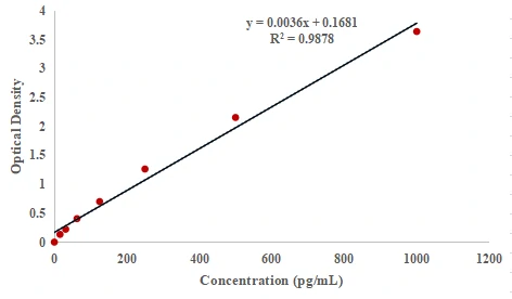
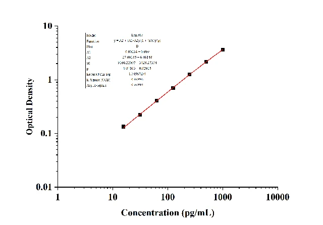
Suppose we have a typical ELISA standard curve with 8 concentration points covering 0–1000 pg/mL.
If the same dataset is analyzed using different models, the results may look very different.

 

Concentration (pg/mL)	OD Value	Predicted Concentration by Linear Regression (pg/mL）	Linear Regression Deviation	Predicted Concentration by 4PL Regression (pg/mL)	4PL Regression Deviation
1000	3.655	968.528	-3.15%	1005.149	0.51%
500	2.168	555.611	11.12%	502.155	0.43%
250	1.277	307.972	23.19%	256.530	2.61%
125	0.714	151.639	21.31%	125.204	0.16%
62.5	0.419	69.556	11.29%	65.389	4.62%
31.25	0.236	18.722	-40.09%	32.658	4.51%
15.625	0.147	-5.861	-137.51%	18.506	18.44%
0	0.013	-43.139	/	0.897	/

For example:
Linear regression:

• R² = 0.9878
• Significant deviation may occur at the low-concentration end
• Maximum relative deviation may become very large

4PL regression:

• R² = 0.99996
• The sigmoidal response is described much more effectively
• Back-calculated concentrations may show substantially better agreement

The important lesson is not simply:
4PL always produces a higher R² than linear regression.
Rather, the correct principle is:
The fitting model should match the biological and analytical behavior of the assay.
For a sigmoidal ELISA standard curve, a nonlinear logistic model is generally more appropriate than forcing the entire concentration range into a straight-line model.

06 Recommended Software for ELISA Curve Fitting

Software	Main advantages	Suitable for
ELISA CALC	Designed specifically for immunoassay analysis; supports 4PL and other models; relatively simple to use	Routine ELISA data analysis
Origin	Powerful curve fitting and customizable nonlinear functions	Advanced data analysis

For routine ELISA analysis, 4PL nonlinear regression is generally a better starting point than simply selecting Excel's linear trendline.

07 Frequently Asked Questions
Q1: Can Excel perform 4PL fitting?
Not directly through the standard Trendline function.
Excel's built-in trendline options include linear, polynomial, exponential, logarithmic, and other basic models, but it does not provide a convenient built-in 4PL nonlinear regression workflow.
4PL analysis can instead be performed using software such as GraphPad Prism, SoftMax Pro, Origin, ELISA CALC, or Python.

Q2: Do I need to generate a new standard curve for every ELISA experiment?
Normally, yes.
Changes in:

• Reagent lot
• Incubation temperature
• Incubation time
• Pipetting
• Washing efficiency
• Operator technique
• Instrument conditions

can affect the assay response.
Therefore, the standards should generally be run together with the samples in each assay run, according to the kit's instructions.

Q3: What should I do if the R² is only 0.96?
Don't immediately assume that the assay has failed.
Check the following in order:
1. Check for outliers
Look for standards whose OD values clearly deviate from the expected trend.
2. Check the fitting model
If you used linear regression across the entire concentration range, try the recommended nonlinear model, such as 4PL.
3. Check the experimental procedure
Review:

• Pipetting accuracy
• Standard preparation and serial dilution
• Washing procedure
• Incubation time
• Incubation temperature
• Substrate development time
• Plate reader settings

4. Check the raw OD values
A poor curve can result from experimental error rather than an inappropriate mathematical model.
Do not simply delete an outlier because it improves R². Any exclusion of a standard should have a predefined and scientifically justified criterion.

Q4: What should I do if the sample concentration is outside the standard curve range?
Do not rely on extrapolation whenever it can be avoided.
If the calculated concentration is above the upper limit of the standard curve, dilute the sample and repeat the assay.
If the concentration is below the lower quantifiable range, depending on the assay and sample type, you may need to:
· Concentrate the sample
· Use a more sensitive assay
· Increase the amount of sample
· Select a kit with a lower detection range
The goal is to ensure that the sample's measured signal falls within the validated quantitative range of the standard curve.

Final Takeaway
ELISA standard curve fitting is not simply a question of “Which method gives me the highest R²?”
A reliable analysis should consider:
Appropriate model → Goodness of fit → Residuals → Back-calculated concentration → Recovery → Precision → Validated assay range
For a typical sigmoidal ELISA dose-response curve, 4PL is generally more appropriate than applying a single linear regression across the entire standard range.
And remember:
A high R² is useful, but R² alone does not prove that an ELISA standard curve is valid.
The most reliable standard curve is one that accurately describes the assay's response and produces acceptable accuracy and precision across the validated quantitative range.